Tutorial
1. Basic usage
In Python interface (include IPython-notebook), user can import flame Machine class.
>>> from flame import Machine
Create Machine object with input file.
>>> with open('lattice_file.lat', 'rb') as f :
>>>     M = Machine(f)
Allocate the beam state. - Machine.allocState(), State
>>> S = M.allocState({})
Run envelope tracking simulation. - Machine.propagate()
>>> M.propagate(S)
The beam state has the finite state beam information. - State()
>>> S            # centroid vector
State: moment0 mean=[7](3.18839,0.00871355,-12.0779,-0.00254204,-35.2039,0.000489827,1)
>>> S.ref_IonEk  # reference energy
11969.995341581
The attribute list of the beam state can be found here.
User can observe the beam state history by using observe keyword in propagate().
>>> result = M.propagate(S, observe=range(len(M))) # observe the beam state in all elements
It returns enumerated list of the beam state.
>>> result[3]
(3, State: moment0 mean=[7](2.2532,0.00489827,2.2532,0.00489827,-2.7162,0.000489827,1))
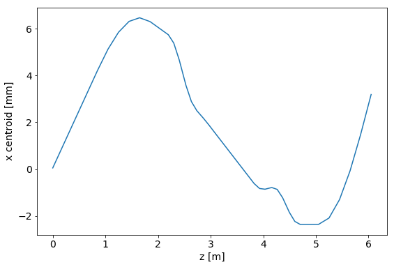
User can generate the history data from the list of beam states,
>>> z = [s[1].pos for s in result] # reference beam position history
>>> x = [s[1].moment0_env[0] for s in result] # x centroid history
and plot.
>>> import matplotlib.pylab as plt
>>> plt.plot(z, x)
>>> plt.ylabel('x centroid [mm]')
>>> plt.xlabel('z [m]')
>>> plt.show()
2. Lattice parameter control
conf() returns initial machine parameter.
>>> M.conf()
OrderedDict([('AMU', 931494320.0),
             ('BaryCenter0',
              array([ 0.1  ,  0.01 ,  0.1  ,  0.01 ,  0.001,  0.001,  1.   ])),
             ('BaryCenter1', array([ 0.,  0.,  0.,  0.,  0.,  0.,  1.])),
             ('IonChargeStates', array([ 0.13865546,  0.14285714])),
             ('IonEk', 11969.995341581),
             ('IonEs', 931494320.0),
             ('IonW', 931506289.9953415),
             ('IonZ', 0.13865546218487396),
             ('NCharge', array([ 10111.,  10531.])),
             ('S0',
              array([  3.68800000e+02,   2.50000000e-02,   0.00000000e+00,
                       0.00000000e+00,   0.00000000e+00,   0.00000000e+00,
                       0.00000000e+00,   2.50000000e-02,   2.88097000e-05,
                       0.00000000e+00,   0.00000000e+00,   0.00000000e+00,
...
User can find the element index by element type or element name.
>>> M.find(type='solenoid')
[15, 16, 18, 19, 21, 22, 27, 28, 30, 31, 33, 34]
>>> M.find(name='q1h_1')
[15]
conf(index) returns all parameters of the element.
>>> M.conf(15).keys() # parameter keywords
['AMU', 'B2', 'BaryCenter0', 'BaryCenter1', 'IonChargeStates', 'IonEk', 'IonEs', 'IonW', 'IonZ', 'L', 'NCharge', 'S0', 'S1', 'aper', 'name', 'sim_type', 'type']
>>> M.conf(15)['B2'] # quadrupole strength
0.942438547187938
Change the parameter by using reconfigure().
>>> M.reconfigure(15, {'B2': 0.8})
Check new parameter of the solenoid.
>>> M.conf(15)['B2']
0.8
3. Run for the selected section
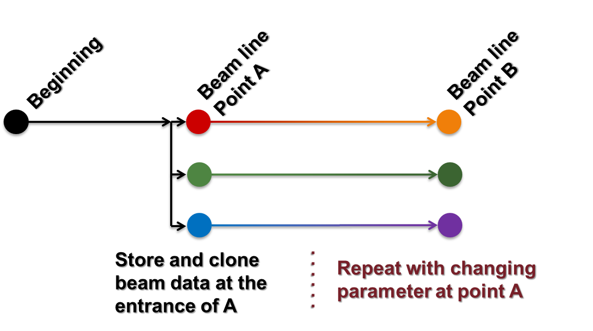
User can input start-point index and propagation number to propagate.
>>> M.propagate(S, 0, 10) # simulate from 0th to 9th element
>>> S1 = S.clone() # clone the beam state
>>> M.propagate(S1, 10) # simulate from 10th to the last element
In this case, “S” has the beam state after the 9th element, and “S1” has the finite beam state.
If user input propagation number as negative number, it returns “backward” propagation result.
>>> M.propagate(S, 0, 101) # forward simulation from 0th to 100th element
>>> S1 = S.clone() # clone the beam state
Here, user can change beam state “S1” except the beam energy and the charge state.
>>> M.propagate(S1, 100, -100) # backward simulation from 100th to the first element
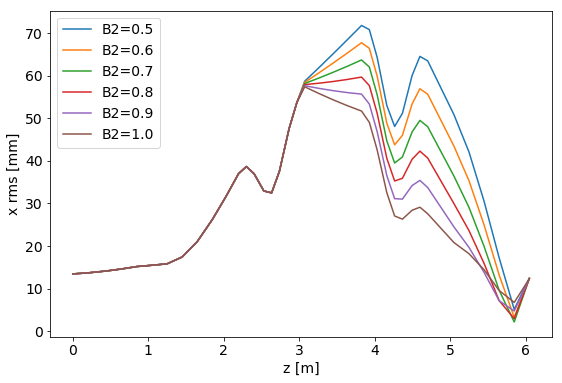
4. Example: Quadrupole scan
Run simulation up to the target element.
>>> M.find(name='q3h_6') # get index of the target element
[22]
>>> ini = M.conf(22)['B2'] # store the initial quadrupole strength
>>> ini
0.853489750615018
>>> SA = M.allocState({})
>>> rA = M.propagate(SA, 0, 22, observe=range(len(M))) # propagate 22 elements from 0
Scan parameters by using simple loop.
>>> b2lst = [0.5, 0.6, 0.7, 0.8, 0.9, 1.0]
>>> rlst = []
>>> for b2 in b2lst:
>>>     SB = SA.clone()
>>>     M.reconfigure(22, {'B2':b2})
>>>     rt = M.propagate(SB,22,-1,observe=range(len(M)))
>>>     rlst.append(rt)
Plot the scan result.
>>> zA = [s[1].pos for s in rA]
>>> xA = [s[1].moment0_rms[0] for s in rA] # get the x rms size
>>>
>>> for b2,rt in zip(b2lst,rlst):
>>>     zt = zA + [s[1].pos for s in rt] # join the history result
>>>     xt = xA + [s[1].moment0_rms[0] for s in rt]
>>>     plt.plot(zt, xt, label='B2='+str(b2))
>>>
>>> plt.ylabel('x rms [mm]')
>>> plt.xlabel('z [m]')
>>> plt.legend(loc='best')
>>> plt.show()